step_profile() creates a specification of a recipe step that will fix the
levels of all variables but one and will create a sequence of values for the
remaining variable. This step can be helpful when creating partial regression
plots for additive models.
Arguments
- recipe
A recipe object. The step will be added to the sequence of operations for this recipe.
- ...
One or more selector functions to choose variables for this step. See
selections()for more details.- profile
A call to
dplyr::vars()) to specify which variable will be profiled (seeselections()). If a column is included in both lists to be fixed and to be profiled, an error is thrown.- pct
A value between 0 and 1 that is the percentile to fix continuous variables. This is applied to all continuous variables captured by the selectors. For date variables, either the minimum, median, or maximum used based on their distance to
pct.- index
The level that qualitative variables will be fixed. If the variables are character (not factors), this will be the index of the sorted unique values. This is applied to all qualitative variables captured by the selectors.
- grid
A named list with elements
pctl(a logical) andlen(an integer). Ifpctl = TRUE, thenlendenotes how many percentiles to use to create the profiling grid. This creates a grid between 0 and 1 and the profile is determined by the percentiles of the data. For example, ifpctl = TRUEandlen = 3, the profile would contain the minimum, median, and maximum values. Ifpctl = FALSE, it defines how many grid points between the minimum and maximum values should be created. This parameter is ignored for qualitative variables (since all of their possible levels are profiled). In the case of date variables,pctl = FALSEwill always be used since there is no quantile method for dates.- columns
A character string of the selected variable names. This field is a placeholder and will be populated once
prep()is used.- role
Not used by this step since no new variables are created.
- trained
A logical to indicate if the quantities for preprocessing have been estimated.
- skip
A logical. Should the step be skipped when the recipe is baked by
bake()? While all operations are baked whenprep()is run, some operations may not be able to be conducted on new data (e.g. processing the outcome variable(s)). Care should be taken when usingskip = TRUEas it may affect the computations for subsequent operations.- id
A character string that is unique to this step to identify it.
Value
An updated version of recipe with the new step added to the
sequence of any existing operations.
Details
This step is atypical in that, when baked, the
new_data argument is ignored; the resulting data set is
based on the fixed and profiled variable's information.
Tidying
When you tidy() this step, a tibble is returned with
columns terms, type , and id:
- terms
character, the selectors or variables selected
- type
character,
"fixed"or"profiled"- id
character, id of this step
Examples
data(Sacramento, package = "modeldata")
# Setup a grid across beds but keep the other values fixed
recipe(~ city + price + beds, data = Sacramento) %>%
step_profile(-beds, profile = vars(beds)) %>%
prep(training = Sacramento) %>%
bake(new_data = NULL)
#> # A tibble: 6 × 3
#> city price beds
#> <fct> <int> <int>
#> 1 ANTELOPE 220000 1
#> 2 ANTELOPE 220000 2
#> 3 ANTELOPE 220000 3
#> 4 ANTELOPE 220000 4
#> 5 ANTELOPE 220000 5
#> 6 ANTELOPE 220000 8
##########
# An *additive* model; not for use when there are interactions or
# other functional relationships between predictors
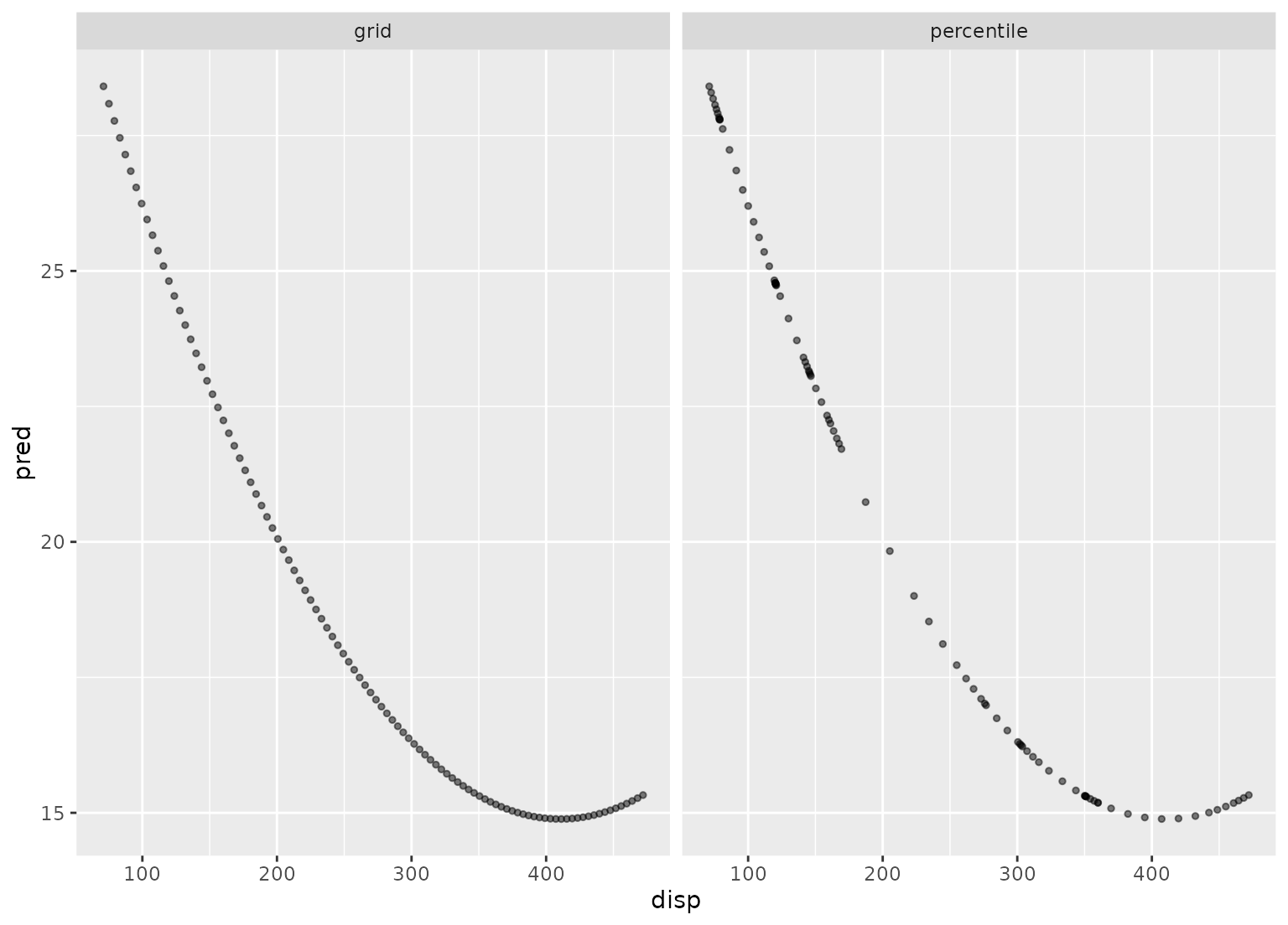
lin_mod <- lm(mpg ~ poly(disp, 2) + cyl + hp, data = mtcars)
# Show the difference in the two grid creation methods
disp_pctl <- recipe(~ disp + cyl + hp, data = mtcars) %>%
step_profile(-disp, profile = vars(disp)) %>%
prep(training = mtcars)
disp_grid <- recipe(~ disp + cyl + hp, data = mtcars) %>%
step_profile(
-disp,
profile = vars(disp),
grid = list(pctl = FALSE, len = 100)
) %>%
prep(training = mtcars)
grid_data <- bake(disp_grid, new_data = NULL)
grid_data <- grid_data %>%
mutate(
pred = predict(lin_mod, grid_data),
method = "grid"
)
pctl_data <- bake(disp_pctl, new_data = NULL)
pctl_data <- pctl_data %>%
mutate(
pred = predict(lin_mod, pctl_data),
method = "percentile"
)
plot_data <- bind_rows(grid_data, pctl_data)
library(ggplot2)
ggplot(plot_data, aes(x = disp, y = pred)) +
geom_point(alpha = .5, cex = 1) +
facet_wrap(~method)